Part 1 - Installing Python

Open science is becoming the standard for reproducible science and many fields have coalesced around several coding languages in support of this. R and Python have seen tremendous use in the academy and for good reason: both are free and open-source with endless packages that extend core functionality that are commonly well documented. This series will work through everything you’ll need to get up and running with Python and even begin doing some basic data manipulation and statistics. In Part 1, we’re going to focus on getting Python installed and running, which we will verify by using Python as a calculator.

There are several ways to install Python and all have their advantages and disadvantages. I’ve found that using Anaconda or miniconda tends to be the easiest and the most user friendly. Anaconda has the advantage of having a graphical user interface, rather than relying on the command line, making it a fantastic entry point for beginners.

What’s the difference between going to Python’s website and installing that version? In terms of the Python installation, very little. However, in practice, Anaconda solves many quality of life issues that plain Python installs have. For instance:

• Aren’t comfortable with using command line tools? No problem! Anaconda has a complete GUI, even for installing packages.
• Want to install a package? Anaconda commonly installs packages a bit faster with less of a headache.
• Want to install a different version of Python? It’s a breeze with Anaconda! Just create a new Python environment and specify which version of Python you’d like to use.
• Want to do spatial data analysis? Gone are the days of dealing with managing to get Python to talk to an OGR/GDAL installation. Anaconda will install Python, OGR/GDAL, and make sure they’re communicating nicely with one another (this is also a huge boon if you use R).

For everything that Anaconda brings to the table there are several downsides. The biggest issue seems to be installing Python modules that are not in the Anaconda repository. If you run into a Python module that is not hosted by Anaconda, you can still install it using pip and PyPi in the command line, but this is usually not recommended. Anaconda likes to manage it’s own dependencies and using pip can break Python environments because Anaconda and pip don’t talk to one another too well. This means that pip may install a version of a module that doesn’t agree with other installed modules. In practice, I’ve found this issue to be quite rare because the conda-forge channel has most modules that any user would need, but it does come up occasionally and there are usually ways around it.

With the background out the way let’s walk through the steps we need to install Anaconda, Python within it, and then write our first Python script.

Step 1 - Download Anaconda

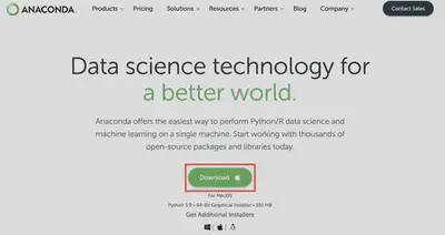
Follow hyperlink at right to download Anaconda.

Step 2 - Install Anaconda

Double click on the .exe (Windows) or .pkg (MacOS) file and follow the prompts to install. No need to make any changes here - the default install settings and location are all okay to use (i.e. just click okay a bunch of times).

Step 3 - Getting Comfortable with Anaconda Navigator

Anaconda automatically creates a base environment with Python and many common tools preinstalled. However, its good practice to create new environments for different projects to ensure that dependencies between modules don’t break code for different projects. For the purposes of this tutorial, we’ll use the base environment that Anaconda creates. However, if you ever create a new Python environment be aware that it comes with minimal modules preinstalled. When I create new environments I typically install the scientific Python stack as it contains the most commonly used functions you will need (NumPy, SciPy, matplotlib, IPython, pandas, SymPy, Jupyter Lab). Though not formally a part of the scientific Python stack I’d recommend also installing Spyder for a good integrated development environment for Python that is an excellent alternative to Jupyter Lab.

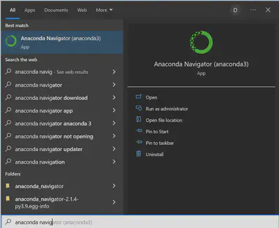
To open Anaconda, search for “Anaconda Navigator” in the Start Menu on a Windows Computer or Spotlight on a Mac.

This is the screen that will greet you when you open Anaconda Navigator:

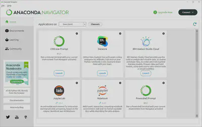
Let’s familiarize ourselves with the layout. The currently active environment is listed to the right of “Applications on” and environments can be easily changed by clicking on the dropdown menu. What we see here are the pre-installed modules and programs in the “base (root)” environment. To view all existing environments, add modules, and manage environments you would click on the “Environments” tab where you should only see a single entry for the “base (root)” environment. We’ll save this for another tutorial, so for now let’s open up the integrated development environment we’ll be using today, Jupyter Lab.

Step 4 - You’re First Script!

Let’s use Jupyter Lab to write our first Python script and plot some data!

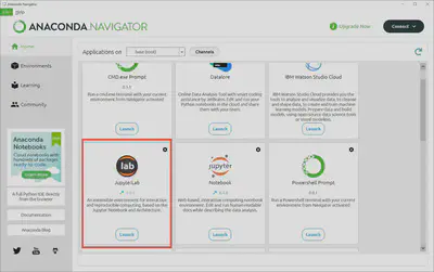
Go back to the “Home” page by clicking on the navigation menu on the left had side of Anaconda Navigator and scroll down until you see the Jupyter Lab logo and a “Launch” button. Click on “Launch” and Jupyter Lab.

That will open your browser and take you’re locally hosted instance of Jupyter Lab. From here we can create a new notebook file (extension .ipynb) and write our first script. But first, let’s change to a dark theme because it’s a bit easier on our eyes and looks nicer.

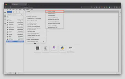
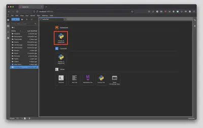
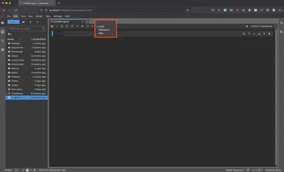
From here click on the “Python 3 (ipykernel) option to create a new Jupyter Notebook file.

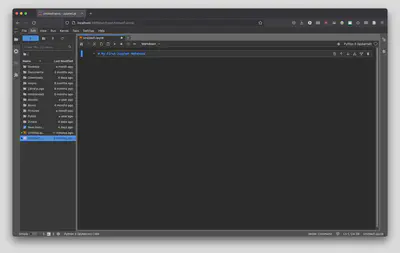
This will be the screen that will greet you when you open a new Jupyter Notebook. Let’s get acquainted with the features of a Jupyter Notebook.

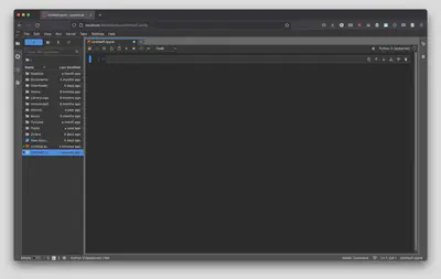
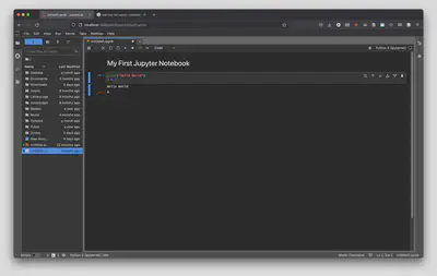
The first empty box you see is called a “cell” and it can contain Python code, plain text, or Markdown code.

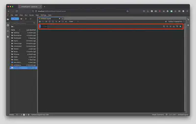
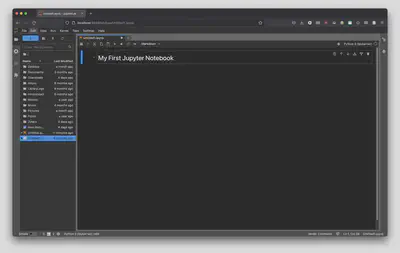
By default, the first cell is defined as Python code, but let’s change it to Markdown and title our first Jupyter Notebook to # My First Notebook.

On your keyboard hit Ctrl + Enter on PC/Linux or Command + Enter on a Mac to render the Markdown cell. Alternatively, you can go to “Run” and select “Render All Markdown Cells”.

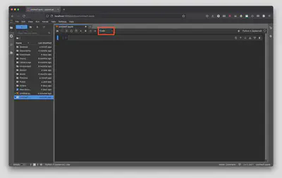
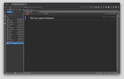
Now that we have a title let’s create a new cell below the title to hold our very first Python code. To do that, click the small plus sign in the top left hand corner of the main notebook interface. Alternatively, you can hit B, B twice on your keyboard. Again, notice how the cell defaults to “Code” which means it will run Python code.

From here, lets use Python to print a message for us by typing in print("Hello World") into the new cell and run the cell by using our keyboard shortcut from earlier (Ctrl + Enter on PC/Linux or Command + Enter on a Mac). You’ll be greeted with a small message below your cell!

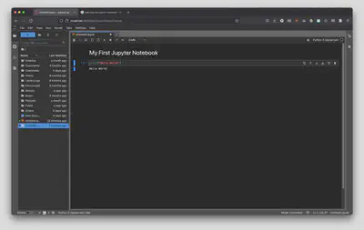
Now, printing “Hello World” isn’t quite scientific computing, so let’s also use this cell as a calculator by typing in 2 + 2 below print("Hello World") and run the cell by using our keyboard shortcut from earlier (Ctrl + Enter on PC/Linux or Command + Enter on a Mac). Once you do that you will be greeted with the answer: 4!

That’s all there is to it! You now have the tools at hand to start writing your own Python scripts and programs for all of your scientific computing needs.

I find that half the battle of starting to learn a new computing language (or anything for the most part) is learning the language. So now that we have a bit of experience with Python let’s finish up with a brief review of some vocabulary we learned today.

Vocabulary

• Anaconda - a tool used to create and manage Python installations (environments)
• Environment - a self-contained installation of Python/R in Anaconda navigator. A single computer can have many environments depending on the needs of the project. For instance, I may want an old Python 2.X environment if I have a tool that only supports Python 2.X.
• Jupyter Lab - an integrated development environment for Jupyter Notebooks
• Jupyter Notebook - an interactive document that can store Python (and R) code, Markdown, and plain text to facilitate open science through the easy sharing of code with the .ipynb file extension
• Cell - the fundamental unit of the Jupyter Notebook, which contains either code, Markdown, or plain text

Part 2 will introduce you to using NumPy, matplotlib, and pandas for ingesting, processing, and plotting data. You can find it here.